In [4]:
from IPython.display import Image
from IPython.core.display import HTML
Image(url= "https://pbs.twimg.com/media/E0JozUlVgAEVeBu.jpg", width=600, height=400)
Out[4]:

In this lecture, we lay out the foundations of statistical inference via hypothesis testing. Hypothesis tests are used to compare two alternatives. For example, hypothesis tests are used in medicine to determine whether a treatment is effective and in genetics to determine whether a certain specific gene is related to a certain, specific trait, or if a specific gene is related to a specific hereditary disease. A lot of scientific discovery comes from hypothesis testing (and reaches media outlets with often exaggerated findings; just search for "power posing" and all the controversy that surrounds it). But not all scientific discovery is accurate. The "wrong" discoveries sometimes happen by chance, and sometimes by manipulating statistical tests. This is one of the reasons why it is so important to understand how different types of hypothesis testing procedures work.
Statistical decision theory provides a framework for making decisions under uncertainty. It encompases both Bayesian and frequentist school of thought (explained later in this section). The basic setup is as follows: we assume that there is some underlying distribution $\mathcal{D}$ that generated pairs of the data $X$ (think of $X$ as multiple data points) and parameter $\theta$, where $\theta$ represents some ground truth (in the case of our binary classification example from last lecture, $\theta$ represented the label $y$ of a data point).
Example 1 Some examples of data $X$ and parameter $\theta$ are:
$X = $ cholesterol level of a patient, $\theta = $ whether or not the patient had a heart attack;
$X = $ monthly rent and $\theta = $ a neighborhood of Madison (e.g., downtown, Willy St/Williamson-Marquette, Dudgeon/Monroe, Shorewood Hills, etc.);
$X = $ thickness of ice on lake Mendota and $\theta = $ one of the months in a calendar year.
Another example of this setup is that the data $X$ we collected comes from a distribution that is fully specified by $\theta$ (here $\theta$ can also be a set of parameters; for example, if the underlying distribution were Bernoulli, $\theta$ would be its probability of getting a 1, if the underlying distribution were Gaussian, $\theta$ would be the mean and the standard deviation, etc.).
A decision procedure is a function $f$ that takes data $X$ as the input and outputs a decision, typically to make inferences about $\theta.$ To determine whether the decision we made was good or bad, we also define a loss function $\ell(f(X), \theta)$ that takes a zero value if we made a correct inference about $\theta$ and some positive value otherwise. For example, in our last lecture, we were talking about constructing a model for binary classification, where the loss function was given by $\ell(f(X), \theta) = \mathbb{1}(f(X) \neq \theta)$ and $\theta = y$ represented the label of a data point $X$.
Where frequentist and Bayesian school of thought differ is in how they treat (the lack of knowledge about) the parameter $\theta$. Both schools of thought assume that $\theta$ is unknown and want to make inferences about it. In the frequentist school of thought, $\theta$ is deterministic ground truth. Even if there were some random event that generated $\theta$, for frequentists, $\theta$ represents what happens on average if that event was repeated infinitely many times. By contrast, Bayesians treat $\theta$ as a random variable. In Bayesian school of thought, $\theta$ is generated from some probability distribution, and, moreover, we know exactly what that distribution (called prior) is.
An alternative way of describing frequentist vs Bayesian perspective is by looking at Bayes Theorem. Both frequentists and Bayesians agree that we can write (by Bayes Theorem):
$$ \mathbb{P}[\theta|X] = \frac{\mathbb{P}[X|\theta]\mathbb{P}[\theta]}{\mathbb{P}[X]}. $$Both assume that you get the data $X$, given $\theta$, i.e., that the data is generated according to probabilities $\mathbb{P}[X|\theta].$ Where they depart is in frequentists making decisions without the knowledge of $\mathbb{P}[\theta]$, whereas Bayesians make decisions taking into account the prior $\mathbb{P}[\theta]$. Frequentists will normally work with $\mathbb{P}[X|\theta],$ i.e., with the distribution from which the data was generated given the parameter $\theta,$ while Bayesians, since they assume the knowledge of the prior $\mathbb{P}[\theta],$ work with the posterior probabilities $\mathbb{P}[\theta|X].$
Both frequentist and Bayesian approaches are useful, but in different settings. Frequentist approaches are generally more robust and are used when there is limited information about the random process that generated the data, or if the decision procedure we are developing is supposed to be used many times, on many different data sets. These approaches are common among computer scientists (and most of what we cover will be from a frequentist perspective). Bayesian point of view is useful when inferences are made by a domain expert who has knowledge or strong beliefs about the random process that generated the data. This perspective is commonly used in areas such as biology, physics, astronomy, etc.
In the simplest (and standard) hypothesis testing setting we have two possible hypotheses: the baseline, that we call "null" (or 0) and the alternative "non-null" (or 1). Scientific discovery happens when we can credibly and correctly reject the null hypothesis, and decide in favor of the alternative. We always assume that there is some ground truth: the reality that we cannot control. All we are trying to do is distinguish between these two possibilities. Of course, mistakes are unavoidable in this process, as we never have the power of perfectly observing the ground truth: all we get are examples that speak in favor or against the null hypothesis.
A quick word of caution: when we talk about decisions here, we will typically assume that the null hypothesis and the alternative are complementary to each other. Thus, when we talk about rejecting the null hypothesis, we can say that we are accepting the alternative. Some statistical tests are performed without these two hypotheses being complementary to each other, and this often complicates things. In those settings, we cannot really talk about "accepting" the alternative; we can just talk about rejecting the null.
As there are two hypotheses (0 and 1) and two cases of ground truth (0 and 1), the following four combinations of truth and decisions are possible
| null decision (0) | non-null decision (1) | |
|---|---|---|
| null truth (0) | true negative | false positive |
| non-null truth (1) | false negative | true positive |
When the decision matches the truth (or reality) we get the "true negative" (in the case of null truth and null decision) and "true positive" (in the case of non-null truth and non-null decision). If the truth is null, but we decide on non-null, this is called "false positive" (a.k.a. Type I error). If the truth is non-null, but we decide on null, this is called "false negative" (a.k.a. Type II error). An easy way to remember what is a false positive and what is a false negative is from this image (source: Twitter)
from IPython.display import Image
from IPython.core.display import HTML
Image(url= "https://pbs.twimg.com/media/E0JozUlVgAEVeBu.jpg", width=600, height=400)
There is often a trade-off between false positives and false negatives, and which ones are more important depends on the context. For example, in the following settings, do you think having low false positives or low false negatives is more important?
(Linear) binary classifiers that we saw in the last lecture are used to classify unlabeled points by assigning them labels "1" and "-1" or "1" and "0" or "+" and "-" (all these are equivalent; we get to decide what the labels mean). Another way of looking at binary classifiers is as decision makers: we decide whether to accept the null hypothesis ("0" or "-1" or "-") or the alternative, non-null hypothesis ("1" or "+"). It is rarely the case that the data can be classified perfectly into positive and negative examples. Hence we can also view the placement of a linear separator that classifies the points as choosing the tradeoff between false positives and false negatives, as illustrated in the following image.
Image(url= "https://storage.googleapis.com/www.jelena-diakonikolas.com/false-positive-false-negative-tradeoff.png", width=400, height=250)

In the last lecture, we did not make a distinction between false positives and false negatives and only focused on minimizing the classification error (the total fraction of false positives and false negatives). It is possible, of course, to set a different goal that would enforce a different tradeoff between false positives and false negatives. One standard approach in hypothesis testing is the classical Neyman-Pearson test (if you saw hypothesis testing in any other classes, you were likely using the Neyman-Pearson test). Before we say what Neyman-Pearson test enforces, we need to introduce a little bit more notation.
It is often the case that we do not perform only one hypothesis test; instead we perform many tests (as in the case when we are classifying points). In such cases, we can consider the counts of true positives/negatives and false positives/negatives, as illustrated in the table below
| null decision (0) | non-null decision (1) | row counts | |
|---|---|---|---|
| null truth (0) | $n_{00}$ | $n_{01}$ | $n_{00} + n_{01}$ |
| non-null truth (1) | $n_{10}$ | $n_{11}$ | $n_{10} + n_{11}$ |
| column counts | $n_{00} + n_{10}$ | $n_{01} + n_{11}$ | N |
One way of looking at whether the decisions we are making are good or not is by looking at correct decisions we are making given the ground truth. These correspond to row counts and are typically used by frequentists. There are two main performance criteria:
There is an inherent tradeoff between sensitivity and specificity. Sensitivity corresponds to the fraction of discoveries we make, given that the non-null hypothesis holds. You can think of it as the conditional probability of deciding on non-null given that the ground truth is non-null. Sensitivity corresponds to not rejecting the null-hypothesis (not making a discovery), given that there is nothing to discover. You can think of it as the conditional probability of deciding on null given that the ground truth is null.
We can artificially make a test very sensitive by proclaiming everything (or almost everything) a discovery (i.e., always accept the non-null hypothesis). Of course, this is not a very good strategy, as it would make the specificity, which corresponds to the fraction of null hypotheses we accept given that the ground truth is null, very low.
As a concrete example of sensitivity-specificity trade-off, consider the following characterization of COVID-19 lab tests from MIT Medicine:
Image(url= "https://medical.mit.edu/sites/default/files/SensSpecTwitter.png", width=800, height=500)
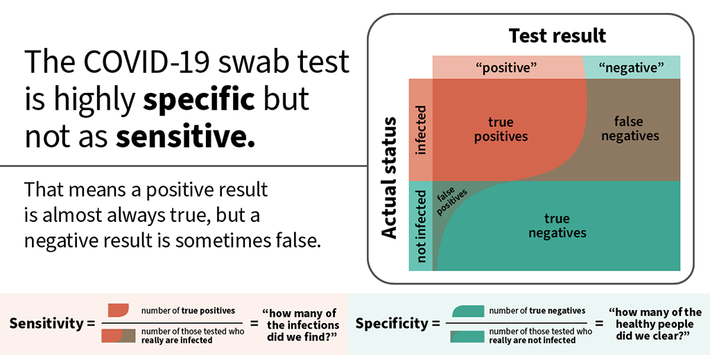
COVID-19 tests have very high specificity but not so high sensitivity, meaning that if you get a positive test it is highly likely that you have COVID, while a negative test does not rule out the possibility of infection so clearly. You have probably heard of this characterization of the tradeoff between false positives and false negatives before, but perhaps have not thought about it coming from the hypothesis testing framework.
We still have not answered how the tradeoffs between sensitivity and specificity (which account for false positives and false negatives) are typically chosen.
In most cases, the choice of tradeoff is determined by what is known as the Neyman-Pearson test. The Neyman-Pearson test sets a significance level $\alpha$ (typically as $0.05$ or $0.01$) and seeks to maximize sensitivity while ensuring that specificity is at least $1 - \alpha.$ We will get back to the Neyman-Pearson framework when we talk about null hypothesis significance testing and p-values in one of the next lectures.
A more Bayesian approach is to consider the column counts, as they correspond to "conditioning on the decision" or "conditioning on the posterior." The relevant quantities are
and
False discovery proportion tells us what fraction of the decisions that we proclaimed discoveries were not really discoveries. It can be thought of as the conditional probability of the ground truth being null, given that we made a decision that it is a discovery. False omission rate on the other hand tells us what fraction of decisions that were proclaimed to not be discoveries were actually discoveries. It can be thought of as the conditional probability of the ground truth being a discovery, given that we decided on null.
Unlike sensitivity and specificity, FDP and FOR depend on the probabilities of the ground truth being null or the alternative. FDP is typically used when we have a belief that most of the ground truth lies in the null, i.e., when a discovery is unlikely.
This lecture is based on Lecture 2 from Data 102 class, as taught in 2019 (by Michael Jordan) and 2020 (by Moritz Hardt). Some of the examples were either constructed by me or taken from the internet (with sources cited in the text).